Fu Lab 
COVID-19
Effectiveness of Massive Travel Restrictions on Mitigating Outbreaks of COVID-19 in China.
Xingru Chen, Xin Wang, Timmy Ma, Daniel Escudero and Feng Fu
Last updated: May 29, 2020
- This report provides preliminary results and is work in progress.
- More detailed results and figures are in the Bag End.
- Original code and data are in the Github Repository.
Abstract
In the very early stage of an unprecedented outbreak of COVID-19 started in the epicenter, Wuhan, Hubei Province, China, the Chinese government imposed by far the largest scale of strict travel restrictions on more than 11 million people (beyond) on January 23, 2020, amid the busiest period of the year for domestic travels (chunyun, travels made during the Lunar New Year). Such massive travel restrictions have caused dramatic reduction in travel volume, not only for the outflow from Wuhan (Hubei), but also nationwide. Control measures like this helps reduce the number of imported cases to other provinces, which can possibly slowdown the onset of epidemic outbreaks in other regions and potentially weaken the impact of the disease. Here, we are interested in estimating the effectiveness of such massive travel restrictions in the mitigation of disease impact using a data driven approach.
Data
The data we used in our research consist of three parts: the COVID-19 infection information, the migration information, and the census in mainland China. We consider the data on a provincial level of 30 provinces (without harming any analysis or conclusion, we do not include Hong Kong, Macau, Tibet, and Taiwan). Notice that the administrative divisions in China are provinces, autonomous regions and municipalities. In this study, they are all referred to as provinces. For the COVID-19 information, we remove all imported (nondomestic) cases from other countries. The start date of our study is
January 15, 2020with the end date beingMar 10, 2020.
Data Source
- COVID-19 information: DXY Pneumonia National Health Commission of PRC Daily Report
- migration information: Baidu Qianxi
- census:China Census Bureau
Data Processing
 |
 |
|---|---|
| (a) A national overview of the epidemic in China. | |
 |
|
| (b) The provincial confirmed cases of COVID-19 by March 10, 2020. We only show the 10 provinces or municipalities most affected by the epidemic. | (c) Growth of the epidemic on the provincial level. The curve in every panel represents the number of cumulative confirmed cases in the respective province and the histogram indicates the number of new confirmed cases per day. |
| (d) Spatial spread of the epidemic by March 10, 2020. The five most affected provinces are highlighted in the map. | |
| Figure 1: Summary of the COVID-19 information as of May 10, 2020. To reduce errors, we have removed all imported cases from other countries. The color in (c) depends on the severity of the epidemic, Hubei being the darkest and Qinghai the lightest. | |
 |
 |
|---|---|
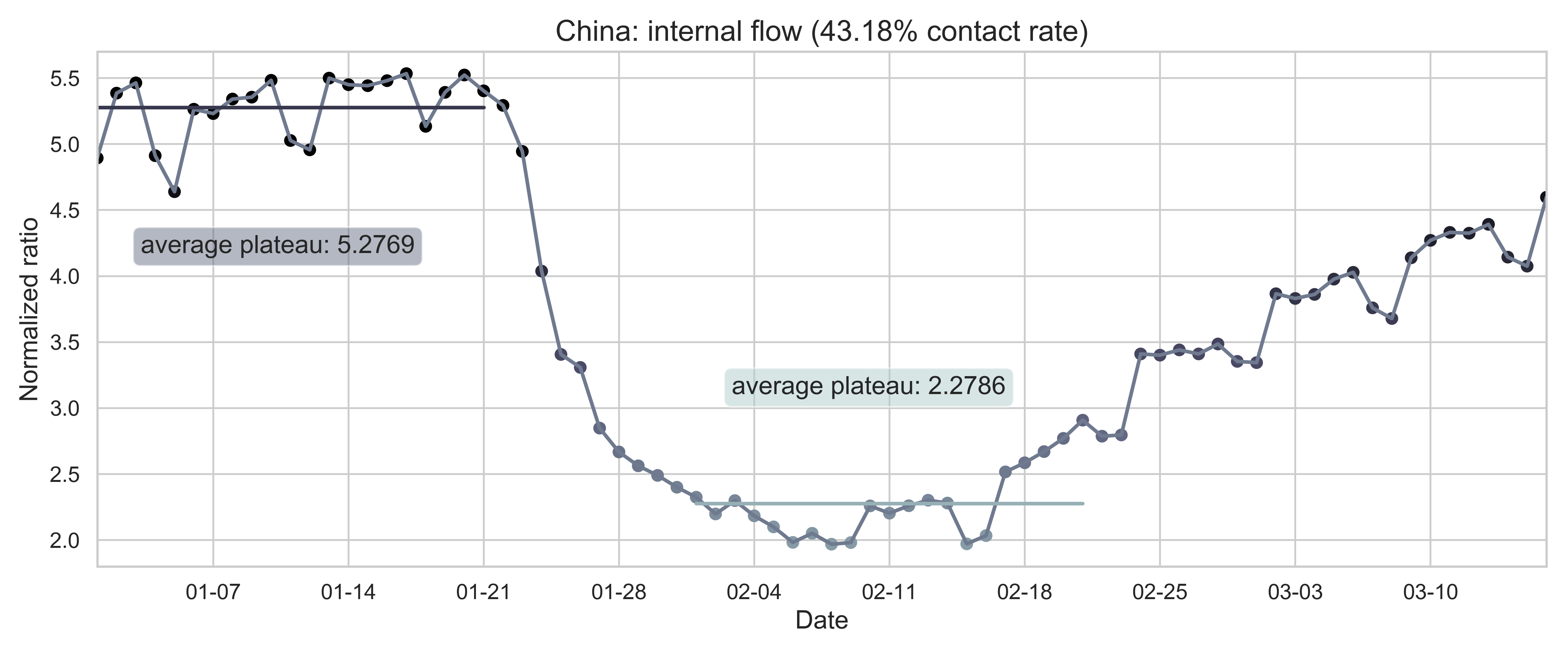
| (a) Nationwide sum of province migration index. | (d) Nationwide normalized internal-flow ratio. |
 |
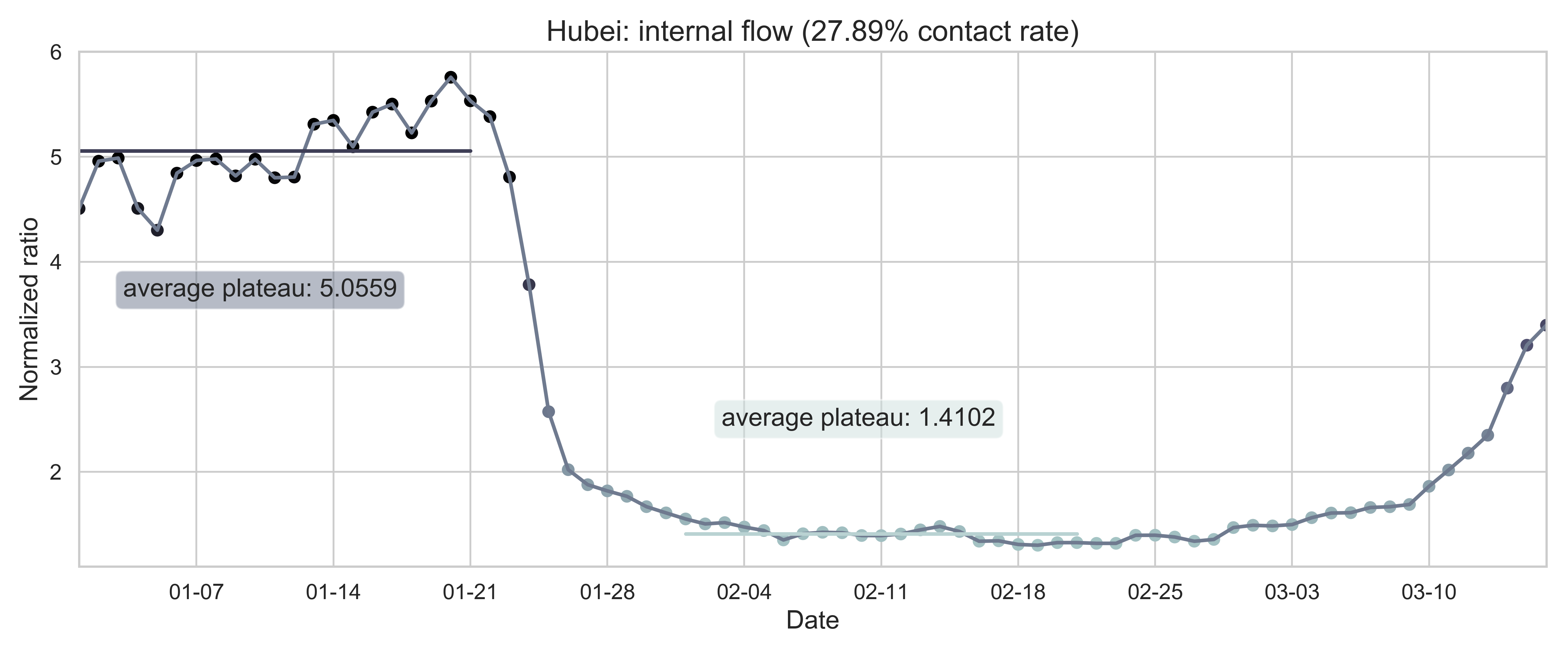 |
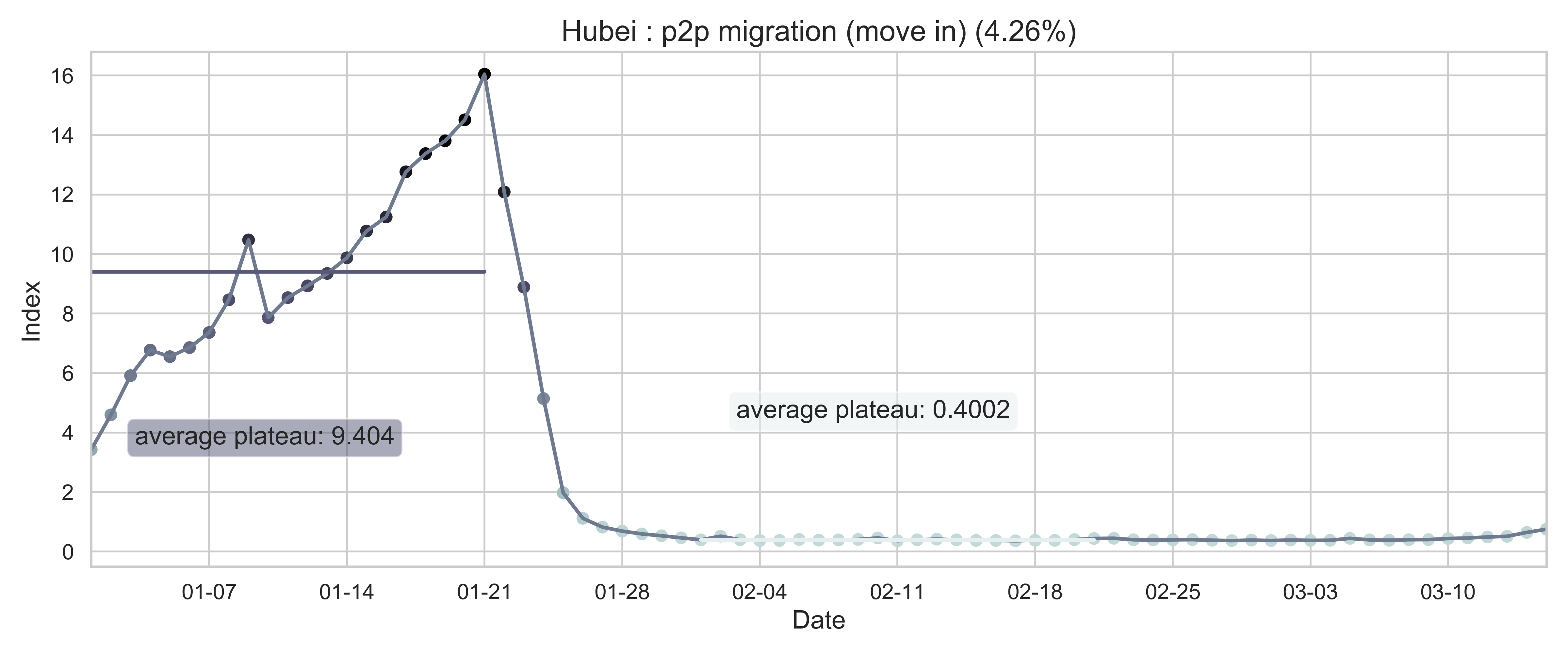
| (b) Province migration index of Hubei (as destination). | (e) Normalized internal-flow ratio of Hubei. |
 |
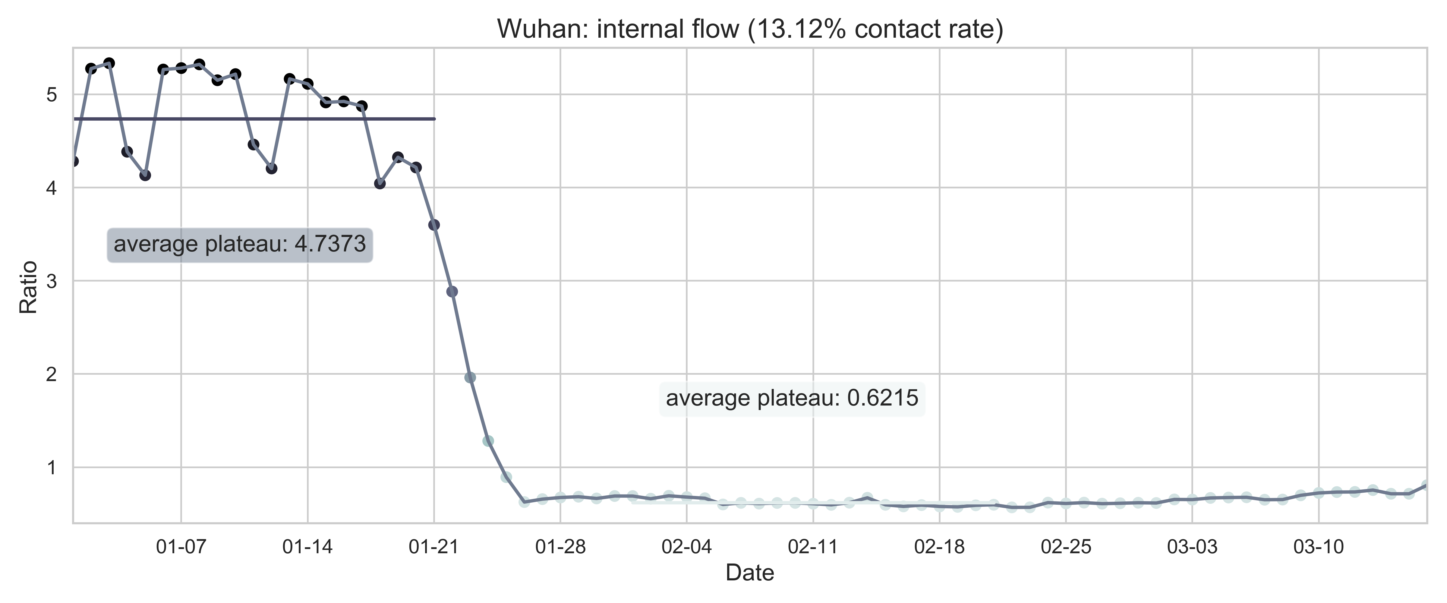 |
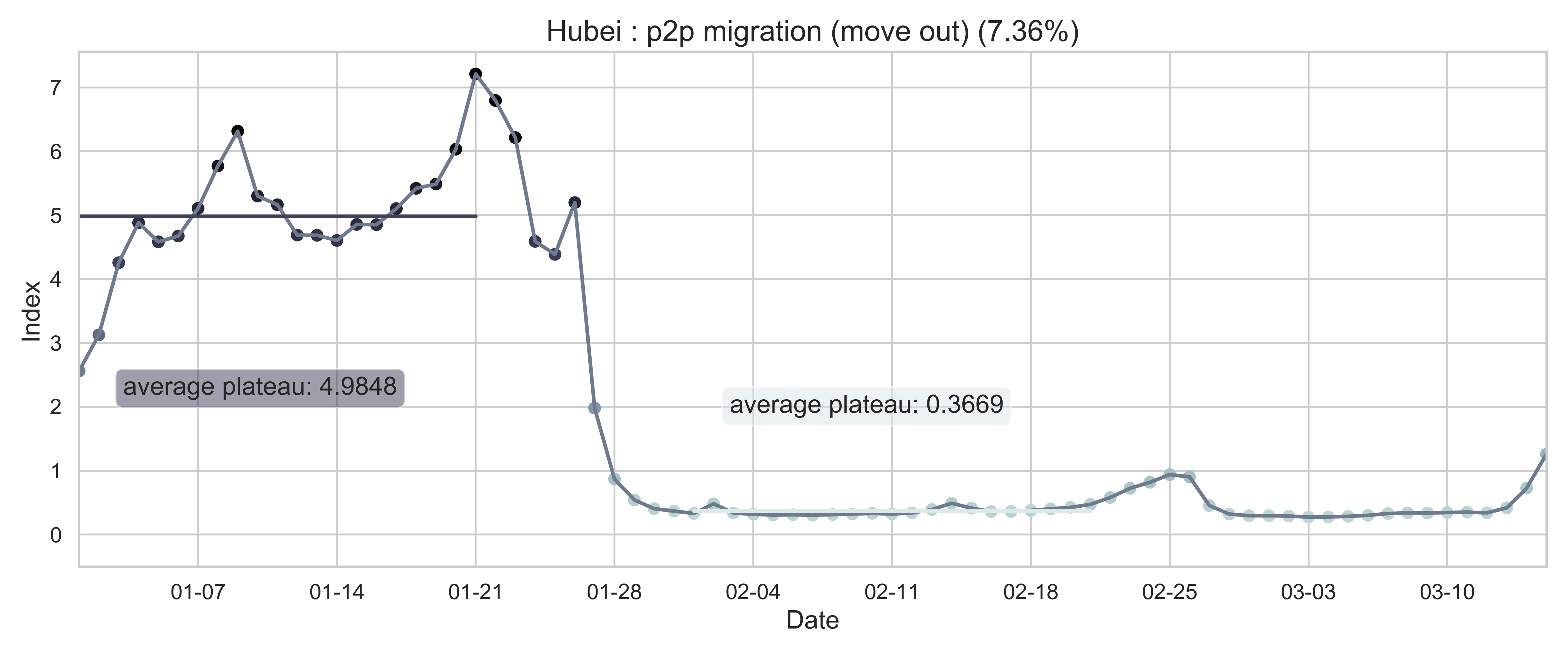
| (c) Province migration index of Hubei (as place of departure). | (f) Internal-flow ratio of Wuhan. |
 |
|
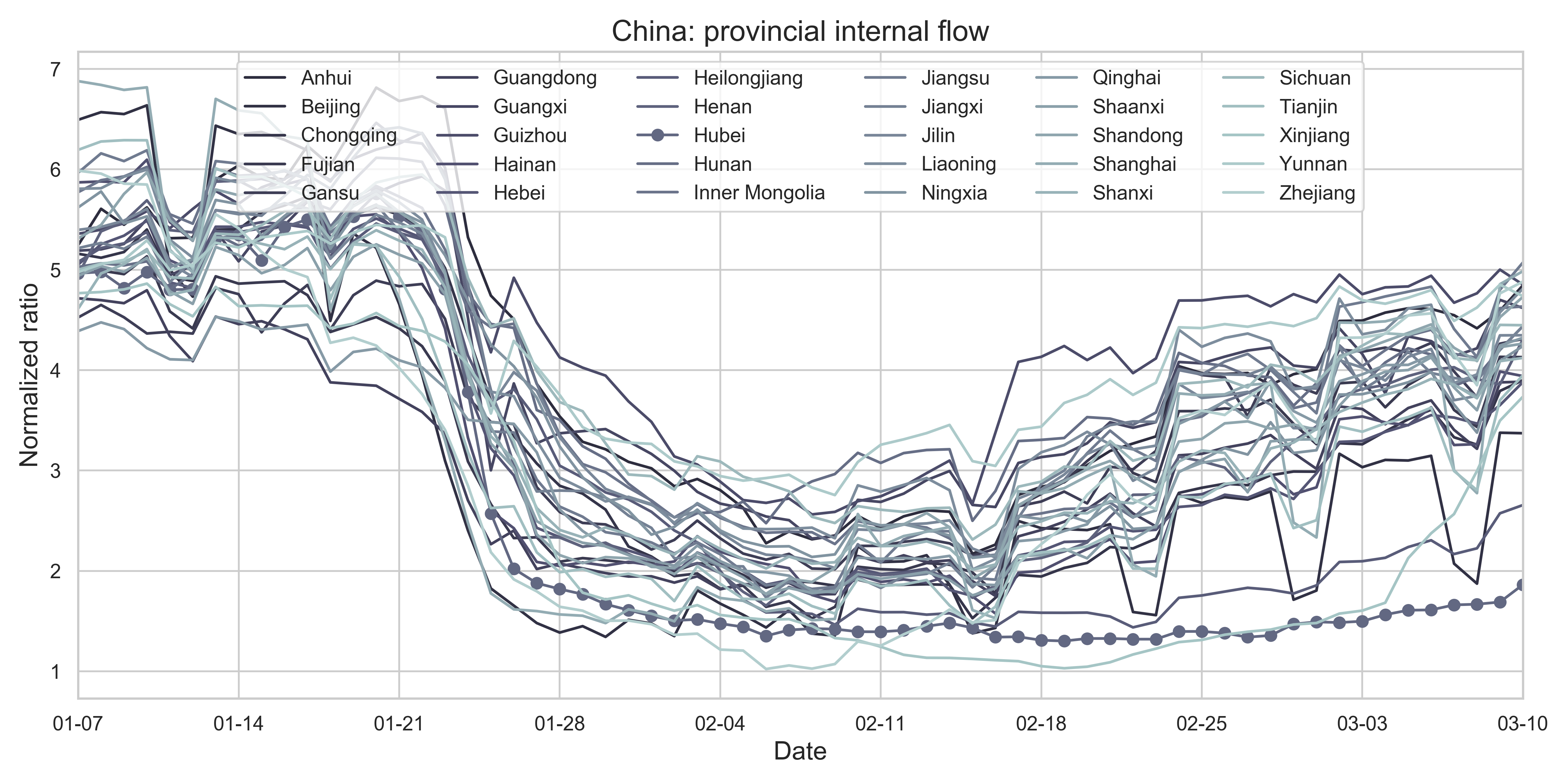
| (g) Provincial level normalized internal-flow ratios. The curve of Hubei Province is highlighted with markers. | |
| Figure 2: Summary of the migration infromation in China, Hubei province and Wuhan city. The time period for calculating the first average plateau value is from January 1, 2020 to January 21, 2020 and that for calculating the second value is from February 1, 2020 to February 21, 2020. For panels (a) - (f), the percentage in the title indicates the after-to-before ratio. | |
 |
 |
|---|---|
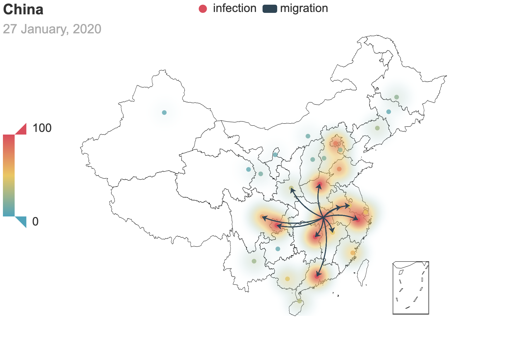
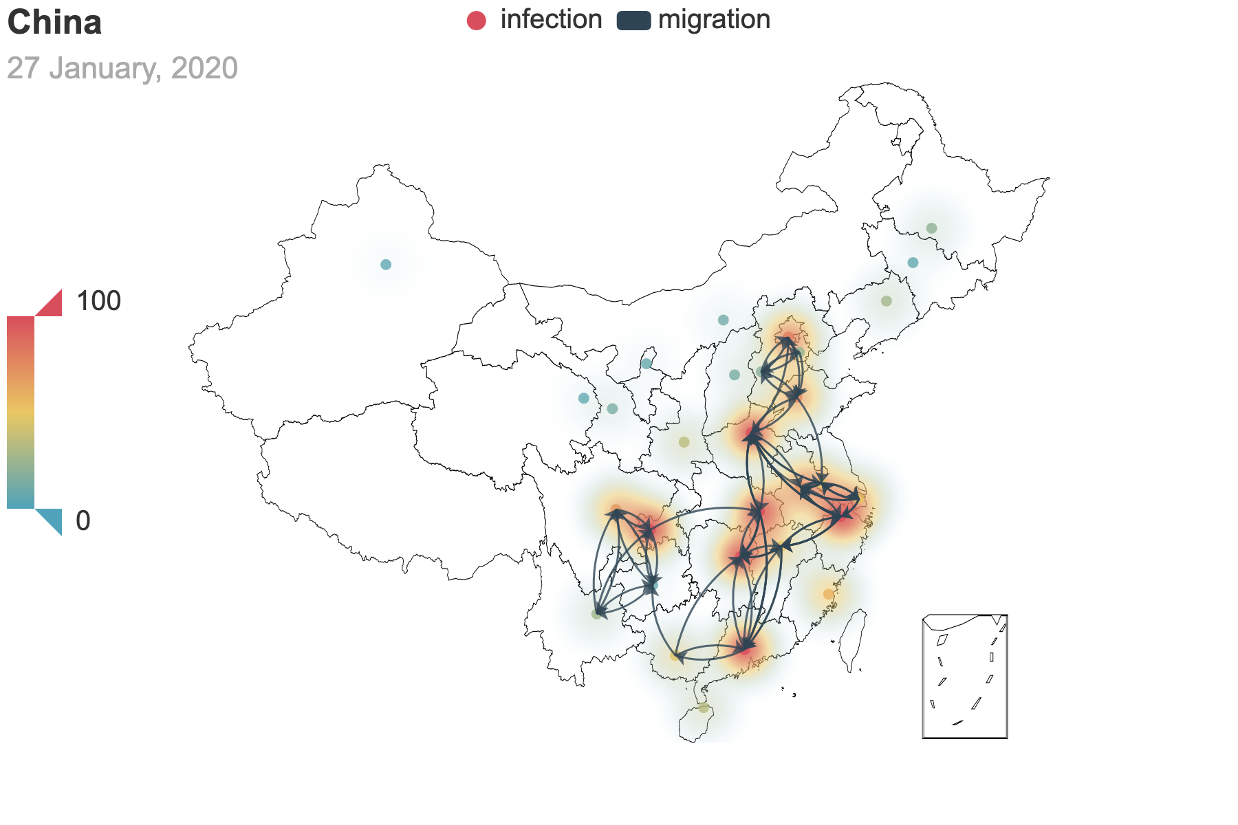
| (a) Migration traces involving the top 10 provinces with the greatest cumulative migration index from the epicenter Hubei Province. | (b) Recursive migration traces involving the top 3 provinces with the greatest cumulative migration index from the departure provinces. |
| Figure 3: Migration traces derived from the migration data. Daily migration index from January 1 to January 27 is added to obtain the cumulative index. And we use heatmap to indicate the number of infected people by January 27. For (b), the first place of departure is Hubei, which points to the 3 destinations: Guangdong, Henan and Hunan. These destinations are treated as the new places of departures and new destinations are added. We repeat this process until there is no new destination appears. | |
Method
SEIR Model
We consider an SEIR model in a meta population structure with migration. The systems of ODEs describe the dynamics in continuous time t, that is, days since the outbreak of the disease:
Here, the subscript $1 \leq i \leq m$ refers to the $i$th compartment on the provincial level (in other words, the $i$th province). $N_i(t) = S_i(t) + E_i(t) + I_i(t) + R_i(t)$ is the total population size of compartment $i$ at time $t$. The total outflow from compartment $i$ to other compartments and the total inflow to compartment $i$ from other compartments are
and
respectively.
To parameterize migration flows between compartments, we utilize the provincial level mobility data from Baidu Qianxi. Notice that the number of confirmed cases by March 10 and the population size of a province differ by at least three orders of magnitude (see the infection rates in the Bag End). Hence $S_i(t) + E_i(t)$ is roughly $N_i(t)$ and we can assume that the following two identities always hold:
Here, $\theta = 100000$ is the unit of p2p migration index.
We further estimate $\alpha_{ij}(t)$ by $\frac{\theta m_{ij}(t)}{N_i(t)}$. A simplified version of the original system of equations is thus obtained:
For convenience, we unify the timeline for all provinces. Since we are using the COVID-19 data from January 15 to March 10, the domain of $t$ in the ODE system can be considered to be $t \in [0, 55]$. In general, all three parameters $\beta_i$, $\sigma_i$ and $\gamma_i$ are functions of $t$. Since $t$ is discrete in practice, we consider these parameters as piecewise functions of which every piece is a constant. In our study, we focus more on the infection rate. After weighing degrees of freedom and flexibility, we assume the following expression where $\beta_i(t)$ is split into twelve pieces, $\sigma_i(t)$ three pieces and the same for $\gamma$:
Parameter Estimation
Prior
Before we include the migration from one compartment to another, we first consider the original SEIR model for every province:
To obtain a prior estimation of the epidemic parameters for the ith province, we apply the dual annealing algorithm to perform a nonlinear least square fitting of the variable $R_i(t)$ and find the global minimum value of the residual. Table 1 shows an ordered dictionary of all the parameter objects required.
| name | initial value | lower bound | upper bound | expression |
|---|---|---|---|---|
| $N_i$ | $n_i$ | |||
| $S_i(0)$ | $N_i - E_i(0) - I_i(0) - R_i(0)$ | |||
| $E_i(0)$ | 50 | 0 | 500 | |
| $I_i(0)$ | 50 | 0 | 200 | |
| $R_i(0)$ | 0 | 0 | 100 | |
| $\beta_{ij}$ | 0.5 | 0.01 | 1 | |
| $\sigma_{ij}$ | 0.5 | 0.05 | 0.5 | |
| $\gamma_{ij}$ | 0.5 | 0.05 | 0.5 | |
| Table 1: Implementation of parameters with reference to the estimations for epidemic parameters. Here, $n_i$ is the population size of province $i$. | ||||
Posterior
After obtaining the prior estimation of parameters for every province, we can further calculate the covariance matrix $\text{cov}(\hat{x})$ and hence the standard errors. The covariance matrix contains complete information about the uncertainty of parameter estimators. To get $\text{cov}(\hat{x})$, we use a linear approximation method through the Jacobian matrix $F$:
Here $s^2$ is the unbiased estimation of the variance $\sigma^2$ obtained from the least square residual:
with $n$ being the total number of measurements, $p$ the number of estimated parameters, $n - p$ the degrees of freedom, $N$ the population size and $S_\text{min}(r, \hat{x}) = \displaystyle\sum(r - R(\hat{x}))^2$ the minimum value of the objective function (that is, the least square residual).
It can be seen from the above calculations that $\text{cov}(\hat{x})$ is a $p\times p$ square matrix. In particular, the diagonal elements are simply the variances of the corresponding ordered parameters (namely, the square root of the $k$th diagonal element is the standard error of the $k$th parameter). Following a student $t$-distribution, we can get the confidence intervals at $(1 - 2\alpha)$ significance for all the parameters and thus their lower and upper bounds:
In our model, we have $n = 56$, $p = 21$ and $n - p = 35$ (notice that $N_i$ and $S_i(0)$ are not free parameters). By letting $\alpha = 0.005$, we obtain the $99.99$% confidence interval of every parameter and for every province. The lower and upper bounds of the epidemic parameters should also be consistent with the sampling of estimations and the lower bounds of $E_i(0)$, $I_i(0)$ as well as $R_i(0)$ should be non-negative. We then get the updated bounds for the parameters:
| name | initial value | lower bound | upper bound | expression |
|---|---|---|---|---|
| $N_i(0)$ | $n_i$ | |||
| $S_i(0)$ | $N_i - E_i(0) - I_i(0) - R_i(0)$ | |||
| $E_i(0)$ | $E_i^{\text{prior}}(0)$ | 0 | $\max(500, E_i^{\text{upper}}(0))$ | |
| $I_i(0)$ | $I_i^{\text{prior}}(0)$ | 0 | $\max(200, I_i^{\text{upper}}(0))$ | |
| $R_i(0)$ | $R_i^{\text{prior}}(0)$ | 0 | $\max(100, R_i^{\text{upper}}(0))$ | |
| $\beta_{ij}$ | $\beta_{ij}^{\text{prior}}$ | 0.01 | $\min(1, \beta_{ij}^{\text{upper}})$ | |
| $\sigma_{ij}$ | $\sigma_{ij}^{\text{prior}}$ | 0.05 | $\min(0.5, \sigma_{ij}^{\text{upper}})$ | |
| $\gamma_{ij}$ | $\gamma_{ij}^{\text{prior}}$ | 0.05 | $\min(0.5, \gamma_{ij}^{\text{upper}})$ | |
| Table 2: Implementation of parameters according to the estimations for epidemic parameters and the results of prior estimation. Still, $n_i$ is the population size of province $i$. The superscripts 'prior' and 'upper' indicate the estimated value and the upper bound from prior estimation. | ||||
Even local optimization methods will be rather time costly under the current situation where we need to solve a giant system of equations, not to mention any global optimization methods. We decide to repeatedly apply the Levenberg-Marquardt algorithm, performing the same nonlinear least square fitting of the variable $R_i(t)$ and finding the local minimum value of the residual. Every time we select a different province and only allow its parameters to be changeable until we iterate through all provinces. To improve the accuracy, we run this iteration process multiple times.
 |
|---|
| Figure 4: Comparison between real and estimated values of $R_i(t)$. The shaded region, the dashed curve and the solid curve correspond to real data, result of prior estimation without migration and that of posterior estimation with migration, respectively. For prior estimation, the maximal number of global search in the dual annealing algorithm is $20000$ and the initial temperature is $10000$. We use the default settings for the other arguments. As to posterior estimation, the iteration defined above is repeated $50$ times. |
Discussion on Parameters
Before we begin our discussion, we would like to emphasize again that there are two aspects of migration: intra-provincial population movements and inter- provincial traffic. For the former, We will see that the intra-provincial migration is closely related to the numbers of initial asymptomatic carriers in provinces other than Hubei. On the other hand, the inter-provincial traffic is highly relevant to the contact rate of a province.
Incubation Seed
We first consider the incubation seed $E(0)$. Here we calculate the cumulative migration index from the epicenter Hubei to any other province between January 1, 2020 (the earliest date for which migration data are accessible from Baidu Qianxi) and January 14 (right before the official record of confirmed cases became available).
 |
|---|
| Figure 5: Prior and posterior estimations of the incubation seed. The provinces in the $y$-axis are ranked according to the severity of the epidemic by March 10, 2020 (the end of our study). The size of a data point for a province other than Hubei is linearly related to the cumulative migration index. A horizontal bar is added for the ith province if $E_i(0)$ shrinks. Given that the number of people should always be an integer, we round up the original values. |
 |
 |
|---|---|
| (a) Migration traces involving the top 10 provinces with the greatest cumulative migration index from the epicenter, Hubei Province. | (b) Recursive migration traces involving the top 3 provinces with the greatest cumulative migration index from the departure provinces. |
| Figure 6: Migration traces based on the cumulative migration index. And we use heatmap to indicate the incubation seed $E(0)$ from the posterior estimation. How we get the places of departure and the destinations in (b) is the same as Figure 3. | |
Contact Rate
We then inspect the contact rate $\beta(t)$.
 |
|---|
| Figure 7: Prior and posterior estimations of the contact rate. There is no significant difference before and after we include inter-provincial migration in the model. The sudden changes later in the timeline may result from the instability of the Levenberg-Marquardt algorithm. |
 |
|---|
| Figure 8: The cross correlation between provincial internal-flow ratio and contact rate. Regarding them as two time series, we calculate their cross correlations with different lags (unit: day) and figure out the maximum value of the correlation coefficient as well as the corresponding lag. Both the coefficient and the lag are given in the title of every panel. Due to the fact that people's travel behavior leads the spread of the disease, we assume that the lag is always positive. |
Infection Number
The last part serves as an addition to the previous analysis. Still, we consider Hubei as the place of departure and calculate the cumulative migration index from January 1 to January 27 (right before the traffic control was in effect).
 |
|---|
| Figure 9: The correlation between province to province migration and infection. Every point stands for a province. The $x$-axis shows when the $10$th patient appeared, that is, at which date our estimated $R_i(t)$ was greater than or equal to $10$ for the first time in the $i$th province. And the $y$-axis represents the cumulative migration index from Hubei to another province. The size of a data point is a linear function of the number of confirmed cases on January 27. |